Java Flight Recorder Demo in JDK 11

Hi, I’m Mark . I’m one of the architects and developers of the JDK flight recorder. Uh, feature included, energetic air lover. I’m going to give you a quick overview of what this feature is, what it is designed to do and give you some hands-on in order to demonstrate how it can assist us solving problems.

What is the JDK flood recorder, the most intuitive way to understand it. Just use the analogy of the recording device in an aircraft, and just like these devices record interesting events related to air travel flight recorders intended to record events related to our programs, what is being recorded, our events.

And we can think of an event as some piece of data at a particular instant of time. Recording events using flight recorder allows us to persist the representation of the execution States in time periods, just before engineering a problem. This entails we can later go back in time. If you will, to understand what was leading up and happen just prior to some problem or less than optimal situation.

The key to flux recorder is being able to record high quantities of information while keeping the overhead of the recording process low, the system is designed to run always on in mission critical environments. Another very important design goal has been to help speed up the time it takes to start the process of problem analysis, thereby cutting the overall time for issue resolution.

Flight recorder tries to accomplish this by recording information that would highlight our system from many different perspectives, ranging from informational overview, such as command line parameters, loaded modules and system properties to some very detailed information regarding say the time waiting to acquire a monitor or the time spent executing a piece of code.

Java Flight Recorder Demo

JVM Profiling with Java Flight Recorder

During subsequent analysis, we can therefore start out from a holistic perspective and drill ever deeper into the relevant details. JFR is especially app for recording latencies, where traditional profiles report time, executing JFR records and reports situation where the application is not executing, or at least not as effective as it could be.

Another design goal is to provide insight into how programs interact with execution environment as a whole, as you are most certainly already aware. Many problems we run into are not directly attributable to logical errors in our programs, but they appear because of a confluence of many factors in relations with flight recorder.

We have a means to capture these usually hard to reproduce situations where a large portion only seems to surface in production environments, the most common and use cases to use GFR as a background recorder, analogous to the recording device in the aircraft. We can also view the flight recorder infrastructure as providing us with an always available profiler, ready to record more extensive information if needed.

And maybe only for a short period of time, they actually interaction with flight recorder is very simplistic. The work we invest is done prior to, and after getting the recording system running in the form of case, we decide our events and metadata using the API. And in the ladder we make use of the recorded information in order to improve our understanding of a system at a particular time or in a particular situation.

And this can be especially helpful in production environments to get data out from flight recorder, we instructed to dump the information that has already recorded, and this produces a binary file, which we can view as a database in compressed format. We can use programmatic API APIs for interacting with this file.

Flight Recorder Java 11

Java Flight Recorder & JDK Mission Control

And this can be useful if you already has some sense of what we’re looking for, but mostly you don’t like any good profile you put to use. It will almost invariably point you somewhere when you had no idea of even start looking in these situations. We can enlist the help of a gooey to assist us manage and better understand the large data sets and relations.

So let’s use J command. We will use Jakeman pit help and we can see five commands for interacting with JFR. The command to start recording is called JFR start

here. I’ve given this first recording a name called continuous, because this will be the recording. We will have running in the background by having this recording running. We can send requests to dump the recorded information anytime we like. And that is exactly what we’ll do here. After letting it record for awhile, we use the JFR dump command to get the information from flight recorder.

So let’s use that here. JFR dump name, continuous file name and let’s call this one discovery dot GFR.

That’s again, issued the JFR check command notice here that the dump operation we just completed is non-destructive in the sense that we still have a background recording running. Now just a quick note on the file, we just dumped a recording file, contains much structure. And this example here, we have a sample file of about five megs in size.

I’ve used the API in JD KJ for consumer to reconstruct the relational information into two standard file formats, Jason and XML, the file size listings, give testimony to the fact that although that the file can be transformed into these other formats, you need to be aware of the size overhead. Now we will start our analysis.

And in order to properly understand the vast amount of information we have at our disposal, we prefer to use a Google tool that would assist us with the analysis process. We will use JDK mission control, which is an excellent tool for doing just this and just us with flight recorder with four JDK, 11 JDK mission control was being open source and donate by Oracle to the open JDK community.

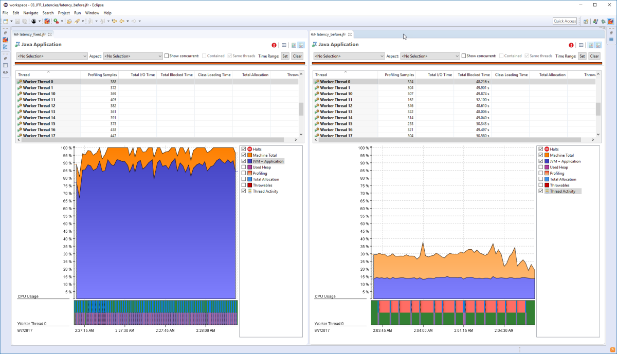
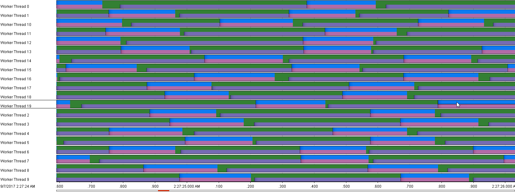
We will be using an early access version of mission control. Let’s click the threads tab here to the left. We can see threads being represented as rows in a table. Each row is projected onto the graph representative execution state. For that particular thread in the graph itself, we can see time plotted along the X axis.

These graphs remind me of sonar graphs. You know, the kind they use in underwater sea bed explorations. And just like Sona graphs help to pick the contours of something we cannot directly observe. So GFR can help us see contours of hard to observe problematic execution patterns. You also see quite a number of red dots.

Flight Recorder Profiling

Java 11, Flight Recorder & Mission Control

These red dots are events. Let’s inspect. What kind of event it is. Java monitor blocked besides giving us. Information about how long this thread was blocked before acquiring the monitor. It also gives us information about the monitor itself. For example, it gives us the instance of the monitor that is represented by the monitor address.

It also gives us the class for this instance, and here it is a Java UTL hash table. In addition, it gives us information about what thread was the previous owner of the monitor when. Monitor blocked events line up like this vertically. It’s a clear indication of a bottleneck. It looks like most threads needs to acquire this particular monitor in order to proceed with execution down the right that is along the time axis.

Let’s select one of these events. Here the stack trace view provides us with great contextual information. We instantly see that this threat is blocked while executing this particular path mission controls or provides another view over unlocks. So let’s check that one as well.

And now let’s check the code related to this.

Why indeed it looks like we’re using a plain old hash table to store our log entries with hash table being synchronized. We immediately see our mistake. Let’s change it to a concurrent hash map. Instead. We’re just about to deploy our new code. What we’re remembered that we might want to turn on JFR from the start.

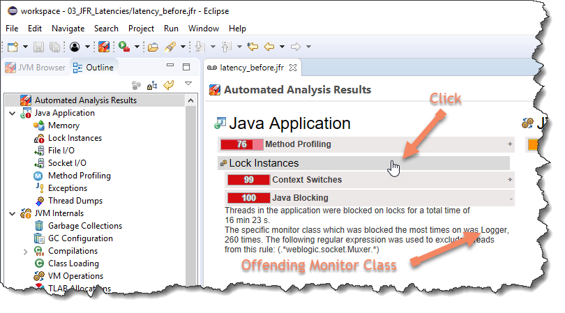
We do another dump for this newly deployed code, which I’m not showing here. And we, again, check the threads tab, look more, no dots. And this example, of course, I knew where to start looking, but sometimes you don’t. The good thing is that mission control can actually assist us with this kind of analysis.

We will redo the same scenario that we just did, but at this time, We will check the automated analysis results. Page one rule here says, look, instances, Java blocking, and it looks like it automatically found the how number of threads being blocked on this particular monitor. Let’s pause here. Why did we not see this into production?

Either we didn’t provoke enough stress during testing to increase the concurrency level to a problematic level. Or maybe we did do that, but we did not use a tool that reported about it during the test cycle. In this situation we were involved with, was it, was it wrong so we could easily change it, but it could just as well as be code located in our library that we were using, we believe GFR can be of assistance here helping us scale this value.

Say we wanted to report this finding to the library developers. We could easily attach this recording to that bug reporting system. Now the bug report just gets stronger. Our arguments backed by empirical evidence. The library developer said their churn is also in a much better position. They have just received a piece of real execution about how their library is being used.

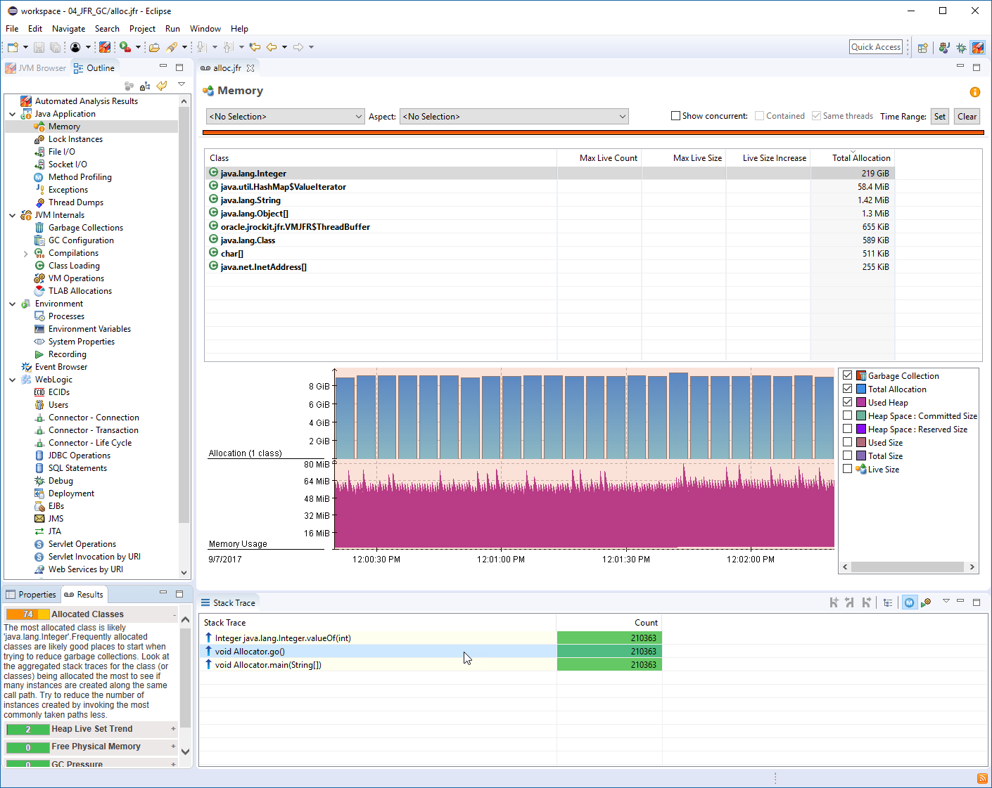
And again, from a production environment. Another philosophical reflection is, but there was no real error involved here. We ended up in a problematic situation because we missed a few details. Let’s see if we can get some additional information from this file. Let’s click the memory tab. What we see here is a salt tooth graph representing heat memory usage in this VM.

Each cycle consists of a build-up phase, which represents a period of heap memory allocations. Followed by a subsequent sharp drop, which are present a GC. And then the cycle starts over. The frequency of this graph seems to be around two Hertz. That is, we have two cycles per second. I respect this in more detail.

eclipse jmc analysis offending monitor

Java performance profiling and JFR

We can see at the start of a cycle, our heap usage is around 500 or seven 70 max at the end of the cycle. Our heap usage has now grown to approximately 2.4 gigabytes. This gives us an allocation, a rate of about four gigs per second. Another valid inference we can make is that most of these allocations are short-lived objects.

The reason for this claim is that the GC is able to push down the heap back to the startup position at each cycle. We can get another piece of important information. If we clicked the garbage collection checkbox. Now it was something with the information, but GC pulse times, what we see is that a GC has a pulse time of about 20 milliseconds.

What this means for us in this context is that the GC stopped our application for about 20 milliseconds to do its work. But since we have two of these GCs per second, we actually have a pulse time of 14 milliseconds per second in this application. At this point, we would like to understand what objects are being allocated and from where GFR provides us with the ability to do object allocation sampling without bytecode instrumentation.

But in order to get this information, we will need to enlist the profiling capabilities of the GFR engine. Since the sampling mechanism has a slight overhead and can generate a lot of data, it does not turn on by default. Instead it is included in our settings for doing a profile recording. We will start an additional recording and we will explicitly pass the settings to do a profile recording to JFR with this heavy rate of allocation, though, we only need to have a very short sample to understand what might be allocating.

So we will also enlist another option. That’s called duration. Which lets us, uh, uh, schedule a time-based recording and let’s just run it for one minute. At the end of this minute, JFR we’ll stop and dump the recording to the file name. We specify. And here we name it allocation, the JFR, we open allocation, JFR and GMC, and we can see that their top section has been populated by information about allocations here.

All the sample instances are grouped according to class. And we can see that the top candidate seems to be a boost array. Quick Mark. Yeah. And Ray, we can see in the stock trace below the actual allocation sites aggregating onto these allocations. And here it seems that there is only one single application site that inspect this code.

This section of the application is involved in calculating prime numbers. And we saw the J for pinpoint of the allocation site for the bullying and race to the line number 35 of the era Toscanini’s algorithm. And here the bullying array has been used as the sifting jury having had this site pinpointed to us, but Jeff, for as being related to high frequency of GCs and consequently of GC Paul’s time.

We can now start to think how it could make this application more effective, maybe by redesigning this piece of code to not allocate as frequently, maybe by using a caching technique or some kind of memoir station. We would be able to much more effective where we’re involved in the analysis of this level.

Performance monitoring anr profiling

It’s very easy to lose track of the bigger picture we might think. Well, what’s 40 milliseconds. We should try to always remind ourselves of the concept of scale. So let’s try to answer this question. What’s the 40 milliseconds, 40 milliseconds per second is 4%. 4% of the time, our application is not doing anything.

It is pause because of GC activity. 4% of 24 hours is almost one hour, 4% of our week is almost Southern hours. So seven hours per week, this application is not doing any useful work. Let’s say we’ve deployed hundred of these instances. So 700 hours per week, our application is sitting idle. Now we feel also had some business model.

We could extend this thought experiment by, by factoring in a monetary value per compute hour. So if we can just figure out a way to maybe have just a single GC happen every second, or that we can get their pulse times down to 10 milliseconds, we would have improved our effectiveness by 350 hours per week.

Closing out this brief demonstration. There’s one more piece that I would like to show you. That’s with JDK nine, we provide Java API APIs that allows you to create your own application specific events into JFR. Although I will not have the time here to demonstrate how to program using the API. I would like to show you an example, what a customer event might look like.

As you remember, my application had a section that evolved calculating prime numbers, and here we can see a custom event. I added two GFR to represent these calculations. There’s a lot of details here that we might need to cover some other time. But the main takeaway message is that there’s no categorical difference between this custom event and the events we’ve been inspecting so far.

Of course, it might look like way, but that is because JMC has predefined views of some of the most general event type. This view also demonstrates another important aspect of GFR. And this is the concept of self-describing data here. James C did not need any particular changes in order to display my custom event.

Instead, the custom event contain the metadata for consumer to represent this information as a specific example. What can I expect the ratio field here? And as you can see, the tool’s able to render this value as a percentage. This has made possible because the customer event has been decorated with Symantec metadata that effectively says to a consumer, this value is a percentage.

So let’s summarize the operator. You shouldn’t, you saw me demonstrate using J co-manager for dump a completely mechanical should I deal with behind it by monitoring tool? Such a monitoring tool could invoke dump operations as a consequence of something happening at the higher level. Maybe a distributed transaction.

If we can expedite the process of getting analysis started most likely through some means of automation, the faster we can understand and solve problems as of JDK nine, Java, API, and Jedi KJ four allow programs to create an integrate their own events. We really hope you like JDK 11. Thank you for watching.